An
Overview Of The CACP Project:
Modelling And Solving
Constraint Satisfaction/Optimisation Problems With Minimal Expert Intervention
Richard Bradwell, John Ford, Patrick Mills, Edward
Tsang, Richard Williams
Department of Computer Science
University of Essex
Colchester CO4 3SQ UK
{rbrad, fordj, millph,
edward, rjw@essex.ac.uk}
http://cswww.essex.ac.uk/CSP/
Abstract
The constraint programming research community
has accumulated a vast amount of experience in solving constraint
satisfaction/optimisation problems. Unfortunately, applying constraint
technology to a particular problem requires expertise in the technology, which
many potential users do not have. The CACP project attempts to provide a system
that encompasses the entire process of applying constraint technology. It supports the tasks of problem formulation
and entry, in addition to supplying pre-written solvers and aiding the user in
choosing which of the available algorithms to apply. Users may specify their
problems using a declarative language. The problem specification is decoupled
from the solvers, so the users may experiment with different problem
formulations easily. Solvers supplied include a generalized Forward Checking
solver, a Linear Programming solver and local search solvers implementing
Guided Local Search, Tabu Search and Genetic Algorithms. A carefully designed
interface is provided to guide users in understanding the technology.
Introduction
Within
the Constraint Satisfaction/Optimisation research community a large amount of
effort has been invested in engineering stronger algorithms, studying problem
difficulty and more recently studying the implications of using different
problem formulations [Tsang 1993; Freuder & Mackworth 1994]. As a result
individual researchers, and the research community in general, have accumulated
a large amount of implicit and explicit domain knowledge regarding how best to
solve problems using constraint technology.
With the knowledge required to apply constraint technology effectively,
it is difficult to transfer the technology to an industrial setting without
requiring an expert in the field.
Knowledge
required to apply constraint technology effectively includes
·
Knowing
how to formulate a problem as a CSP/COP.
·
Knowing
how to engineer a solver.
·
Knowing
a good formulation for a given problem.
·
Knowing
which solver to apply to a given problem.
·
Knowing
how to incorporate domain knowledge into the solver.
Various
industrial strength packages, e.g. ILOG Solver, have been implemented with the
explicit aim of making access to constraints technology easier
(http://www.ilog.fr). Even packages
such as these require a large amount of expertise because they usually come in
the form of a constraint library that can be linked to a standard application,
written in the desired 3GL. Knowledge of
the target language and the constraint library is still required. Generally they concentrate only on the issue
of solving, relieving the user from the burden of writing their own solver.
The CACP
project attempts to provide a system that encompasses the entire process of
applying constraint technology. It
supports the tasks of problem formulation and entry, in addition to supplying
pre-written solvers and aiding the user in choosing which of the available
algorithms to apply. Problems are
modelled in the declarative EaCL language, which the user can enter via an
intuitive user interface. The problem specification is decoupled from the
solvers, so the users may experiment with different problem formulations
easily. Careful attention has been directed to providing a user friendly
GUI based system for easy entry of problem constraints. An extensive help system is also provided.
Having formulated the problem in the EaCL language and entered the problem, the
user can solve the problem using one of the pre-written generic solvers. Choosing the correct solver from a problem
is often a difficult task and therefore the CACP project makes an initial
attempt to address this issue also.
Within
the research community competition between algorithms drives researchers to
produce faster algorithms that produce better results, for a restricted set of
problems. Generally this is
accomplished by tailoring the algorithm using large amounts of domain
knowledge. The goal of the CACP project
is not to compete with these highly specialised algorithms. In many industrial settings solutions are
produced manually and a large amount of time and effort is invested in
producing those solutions. Any solution
to the problem, provided by a highly automated, easy to use system, produced
within a reasonable time frame is usually what is desired. This is the premise on which the CACP
project was built. The system implemented is primarily targeted for users who
are not interested in implementing constraint programming techniques, but would
like to exploit constraint technology.
Architecture
The CACP
architecture is given in Figure 1. The
main flow of control starts with the entry of the problem definition in a
language developed within the group, named EaCL. Additional data, required for more demanding problems, can be
read in automatically from Excel by using it as an automation server. Problem description entry is performed using
either the ZDC or ZDC Direct user interface.
ZDC Direct allows the user to enter the problem formulation as
text. ZDC uses a more elaborate
interface to shield the user from the EaCL grammar, making problem entry
easier.
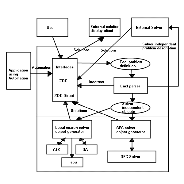
Figure 1:
The CACP Architecture
Once a problem description has been entered by the user, the EaCL
parser parses the description. An
invalid formulation is reported back to the user via the user interface. A correctly parsed definition generates the
raw, solver independent constraint objects.
These solver independent objects are use by the selected solver as a
guide to generate its own set of constraint objects. This architecture essentially separates the solver and its object
library from the parser, allowing the architecture to be easily extensible. It is important to allow this separation
because EaCL potentially supports a large number of different problem
types. Each solver specialises in
solving a particular class of problem and therefore requires a different set of
constraint objects from solvers solving other problem types.
An
algorithm selection expert module is responsible for matching the problem
formulation to the available solver algorithms that can potentially be applied
to that formulation. A solver, when
invoked, runs in a separate thread, with only one thread executing at a
time. The thread terminates once the
solver has found a solution, or the solver has been terminated
prematurely. The results from the
solver are passed back to the user interface, where they are relayed to the
user. Described above is the normal
usage of the system. ZDC can also perform the role of an
automation server. This means that
standalone applications with specific user interfaces can be written for a
particular domain, yet as automation clients they can access some of the
problem solving capabilities of ZDC.
The group, to demonstrate this feature, has developed a timetable
planning application.
ZDC can
also perform the role of a problem description server, using sockets. This means that ZDC can provide an external
solver with a description of the variables, domains and constraints of the
currently parsed problem. This
facilitates a greater separation between the two separate phases of problem
modelling and solving. The EaCL Parser
generates a solver independent description of the problem. The description instructs the external
client solver how to generate a constraint object tree, using its own
constraint object library. The
separation of modelling and solving is useful for a number of reasons. Firstly, it becomes very easy to add
additional solvers to the system.
External solver clients register with the server and the server becomes
aware of their existence. An external
solver can submit itself as a slave solver by sending the appropriate message
to the server. As a slave, the external
solver is under direct control of the server.
The user can interact with the ZDC interface and force an external
solver to solve the current problem being modelled and then return the results,
as if it was an internal solver.
A number
of external solvers, registered as slaves, can be instructed to solve the same
problem at the same time. The use of
the client/server model using sockets allows external solvers to be separate
processes, possibly running on different machines over a network. Solutions, when received from the external
solvers by the server, are stored for later viewing by the user. External
solvers do not have to submit themselves as slave solvers. They can work
autonomously and control their interaction with the server. In this manner the external solver can use
ZDC as a problem description provider or solution displayer. GLS and its constraint object library have
been externalised, to demonstrate the client/server architecture.
We intend
to modify the server so that it can support different types of clients to be
register with the server. It would,
for example, be desirable to provide clients that display solutions in a manner
appropriate to the problem being solved.
The server will send solutions, when produced, to all registered display
clients. Only those capable of
displaying the solution will do so. To
summarise, the CACP project, through its use of automation and sockets provides
an open architecture. This allows
applications to exploit the existing framework and tailor it more to a specific
application domain, if required.
Problem Modelling in EaCL
The Easy
abstract Constraint Optimisation Programming Language (EaCL) is the language
used to formulate problems prior to solving.
A valid problem formulation is split into data, domains, variable,
constraints and optimisation sub-sections.
EaCL supports variables with integer, boolean, real and sets as
domains. The EaCL grammar supports a
wide range of logical, integer, set and symbolic constraints. There are also various facilities supporting
lists and sets as well as conditional branching. For a complete description of the EaCL language consult [Mills
et al 1998]. Modelling problems is one
of the core activities and the main strength of the CACP project. For this reason we present an in-depth
tutorial, demonstrating how to model a number of well-known test-bed problems
in the Appendix.
The Algorithm Expert
Providing
a system that allows multiple solvers is strength in the sense that it allows a
larger array of problem types to be solved by the system. Even having multiple solvers that are
applicable to the same type of problem is advantageous because it allows
greater scope for solving a given problem successfully. The weakness of maintaining a portfolio of
algorithms is that it introduces additional choice to the user. Choosing the correct algorithm potentially
requires a large amount of domain expertise.
To simplify the choice it is suggested that an algorithm expert be
used.
The
algorithm expert is a function which, given a particular problem instance as
its input, identifies from the portfolio of algorithms those which are
applicable to the problem type. A
secondary function of an algorithm expert is to take the set of algorithms
applicable to the current problem class and reduce it further to the set it
believed to perform best for the current problem instance. The first task in selecting a suitable
algorithm is to reduce the set of algorithms based on the type of problem. A heuristic is incorporated in ZDC, which identifies
Linear Programming (LP) problems and allows only the Simplex method to be
applied to those problems. For other
problem types such as problems containing variables with discrete domains, all
of the incomplete heuristic based algorithms and the GFC algorithm, can
potentially be applied to solve these problems.
Once a
set of algorithms has been identified according to the problem type there is
the possibility of further reducing the choice of algorithms. ZDC takes a pragmatic approach to algorithm
selection by switching between algorithms mid-run if it is found that the
current algorithm is in effective.
When switching takes place no solutions are passed between algorithms
and each algorithm restarts from a new random solution. A single run involves trying all applicable
algorithms in a given order until one of the algorithms succeeds in returning a
valid solution, or the list of algorithms is exhausted. The algorithm expert attempts to predict
based on previous runs, the probability of success for each algorithm and then
orders them in the run accordingly to its predication. The solvers the algorithm expert believes to
be the most promising are applied early in the run so there is a greater chance
of early successful termination. This is partly based on the assumption that a
user is likely to use ZDC to solve similar types of problems.
As a
first attempt, the algorithm expert has been implemented to select its
preferred algorithm ordering probabilistically, based on how well the
algorithms have performed in the past.
A simple weight is maintained for each algorithm. Roulette wheel selection is used to select
the ordering of the algorithms using the algorithm weights. An algorithm’s weight is used as its slot
size in the selection process and algorithms that have previously performed
well have a large slot size biasing the selection process towards them. A heuristic built into the expert ensures
that GFC is always ordered first in the run, based on the observation that an
exact search should take precedence over an incomplete search. Knowledge can be built into the individual
solvers to identify when they are making insufficient progress and they can
terminate before the end of their allotted “time slice”. The forward checking algorithm [Haralick
& Elliott 1980] has been implemented with a thrashing detecting mechanism
developed in [Borrett et al 1996] for detecting if the search is
thrashing. How to detect if an
incomplete search algorithm is unlikely to make any further progress is still an
open research area. Therefore, at
present, we have no corresponding heuristic for the incomplete methods.
The Solvers
A number
of generic solvers have been implemented within the CACP framework. Firstly, a simplex algorithm is used to
solve problems containing variables with real domains. A Generalised Forward Checking (GFC)
algorithm has also been implemented, with a corresponding library of constraint
objects, to represent the complete search algorithms. The forward checking algorithm, when applied to an optimisation
problem, maintains the best solution cost and uses it as a bound on the current
solution cost. GFC has also been
extended so that it can be applied to problems involving n-ary constraints. As mentioned previously, built into the GFC
algorithm is a thrashing detection mechanism that detects if the solver is an
inefficient method for solving the current problem. Upon detection of thrashing the GFC is automatically terminated. Three local search techniques have been
implemented, all sharing the same library of constraint objects. The solvers implemented are a Genetic
Algorithm, Tabu Search and Guided Local Search. Initially we focus on GLS in detail because it demonstrates some
of the principles used in the other algorithms.
The Guided Local Search Solver
Guided
Local search (GLS) [Voudouris & Tsang 1999] is a meta-heuristic. When the hill climber is
caught in a local minimum it provides a mean of escaping the local
minimum. Essentially GLS escapes from
a local minimum by adding extra penalty terms to the cost function. When the algorithm detects it is in a local
minimum it chooses a feature of the current solution to penalise. A term is then added to the cost function to
increase the cost of any solution containing the penalised feature. Penalising the feature results in an
increasing in the cost of the local minimum. Neighbouring solutions that do not
exhibit the penalised features become more desirable, and hill climbing
re-commences.
GLS has
been implemented, in the project, to choose a downward move at random if one is
available. A move is defined as
unlabelling the chosen variable and re-labelling it with a different
value. A downward move is one that
reduces the number of conflicts the chosen variable is involved in. If no downward moves are available, then
random sideways moves are tried. After
a small number of consecutive sideways moves the escape mechanism is
activated. The escape mechanism
penalises features to escape local minima.
In the context of constraint satisfaction, candidates for penalisation
should be related to the current constraint violations. The variables involved in a constraint
violation and their corresponding labels are used as features.
In an
effort to speed up the GLS algorithm there are options to ignore constraints of
arity greater than four. There is an
additional option that allows only those constraints initially violated to be
considered. The remaining constraints
are only considered when a solution is found that does not violate those
constraints initially violated.
Label Inputs Table
A necessary
step of local search is to examine the candidate neighbouring solutions. The
GLS and Tabu Search (to be elaborated later) implementation maintains a table
called the label inputs to make this task easier. The label inputs table holds, for each variable, the output of
the constraints for each possible label in the variable domain. In effect the list indicates the number of
conflicts a variable will be involved in if it is relabelled, for all domain
values. The effects of the objective
function are also added to the label inputs when solving optimisation
problems. An example of how exactly
the label inputs are calculated is given below.
Figure 2
formulates a simple problem in EaCL.
The formulation describes a problem with two integer variables a and
b. The product of the two variables is
constrained to equal to a target value.
The sum of a and b is minimised.
If random labels are chosen for the variables then the label inputs can
be calculated. For example, if a and b
have the values of two and five respectively then the corresponding label
inputs are give in table 1. Each column
in the table represents a variable.
Each row in the table represents a variable labelling. For example, the contents of cell (b, 6)
indicates the amount the constraint would be violated if b was given the label
value six. We notice that this change
would reduce the constraint input of variable b from its initial value of 1630
to 666. This is not surprising because
labelling variable b with the value of six satisfies the constraint. The actual values given in the table cells
need further explanation.